Input Files¶

ALLCools Starts From Mapped Data¶

ALLCools is designed for post-mapping data preprocessing data analysis. Therefore, our tool starts from the mapped and demultiplexed data. Please refer to the data provider or corresponding methods/pipelines for demultiplexing single-cell reads and mapping them on to the reference genome.

Note

For all the data generated by snmC-seq and related single-cell multi-omics technologies in Ecker Lab, we use the YAP pipeline to demultiplex and map the reads. YAP uses bismark to map reads and generate single-cell ALLC files from each filtered BAM files.

After demultiplexing and mapping, you will get one BAM file per cell containing sorted and uniquely mapped reads. From each BAM file, you can create one ALLC file using allcools command line tools.

Data Analysis Starting From Core File Formats¶

We use three file formats to store cellular analysis and genomic analysis data.

File Format	Analysis Level	Genome Resolution	Data Type	mC Context	Matrix Form	Based On
ALLC	Cellular	single base pair	raw counts	all mC context	N.A.	tab-separated table, compressed by bgzip, indexed by tabix
`MCDS`	Cellular	genome regions	raw counts & miscellaneous	multiple user-defined mC context	N-D Dense Matrix	`xarray.Dataset`
`RegionDS`	Genomic	single base pair to large genome regions	raw counts & miscellaneous	miscellaneous	N-D Dense Matrix	`xarray.Dataset`

Relationships between three data file formats¶

The ALLC files are generated from the raw sequencing data, containing the base-level cytosine counts (raw data). Subsequently, the MCDS file is generated from a set of ALLC files. The MCDS file is the starting point of cellular analysis (cell-by-region matrix). The RegionDS file is the starting point of genomic analysis (region-by-annotation matrix).

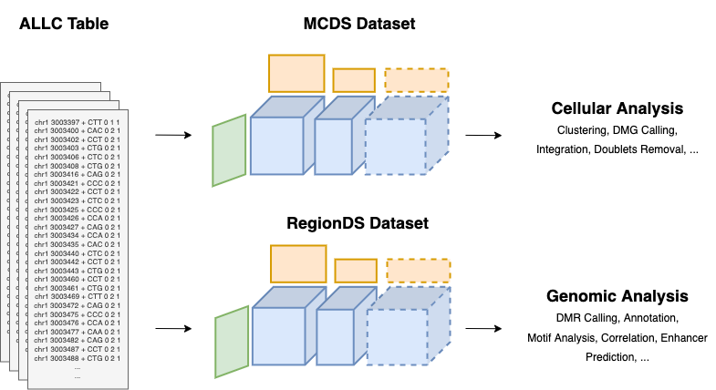
Fig. 3 ALLCools data model for handling single-cell methylomes and performing cellular and genomic analysis.¶

Base Resolution Count Table¶

ALLC File¶

The ALLC (ALL Cytosine) format is a tab-separated table containing base level methylation and coverage counts. This format is originally defined by methylpy, a python package developed in the Ecker lab for bulk WGBS-seq data analysis. Each row in an ALLC file corresponds to one cytosine in the genome. An ALLC file contains 7 mandatory columns with no header. ALLCools assumes all the ALLC files are compressed and indexed by bgzip and tabix from the htslib [Li, 2011]. The ALLC file generated from a single-cell BAM file only contains information from a single cell. Multiple ALLC files can also be merged into an ALLC file (e.g., merge by cell cluster) as a pseudo-bulk-level methylation table.

For more details on generating and handling ALLC files, please read the introduction of allcools command line tools.

Columns in ALLC file¶

index	column name	example	note
1	chromosome	chr12	chromosome names need to be the same as genome FASTA
2	position	18283342	1-based
3	strand	+	either + or -
4	sequence context	CGT	can be more than 3 bases
5	mc	1	count of reads supporting methylation
6	cov	2	read coverage
7	methylated	1	indicator of significant methylation (1 if no test is performed)

Compression and Indexing ALLC¶

All the ALLC files generated by ALLCools are compressed by bgzip and indexed by tabix. The tabix enable us to query ALLC files with specific genomic regions. To check whether your ALLC files meet the standard, you can use allcools standard to validate the compression and indexing. You can also use allcools tbi to index ALLC files using tabix.

Tip

bgzip and tabix [Li, 2011] are wonderful tools to compress tab separated tables with genome coordinates. Because it allows accessing any parts of the compressed file by genome location or region, which allows allcools to perform many region level parallelization in its file handling commands.

Cell-by-feature Methylome Matrix¶

For cellular analysis like clustering, we need to first aggregate the base-level methylation information into the region-level and gather thousands of cells together into a data matrix. To do so, we provide MCDS format to store all kinds of quantification outlined below.

MCDS File: N-D dense matrix for raw counts¶

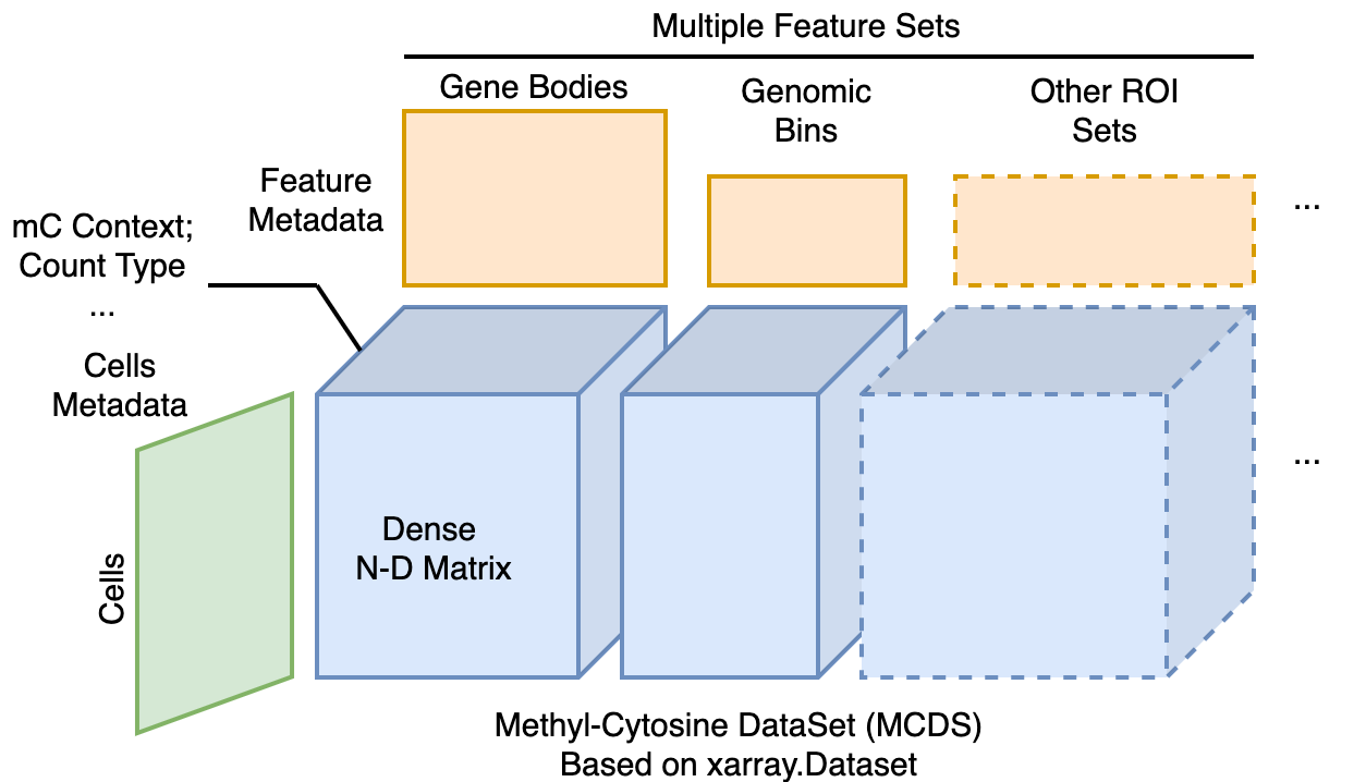
Fig. 4 Schematic of one MCDS file.¶

Here are some design principles for MCDS format:

Raw count matrix in MCDS¶

The MCDS is a versatile data matrix format for storing region-level methylation values from a set of cells. It can handle all sizes of regions (from hundreds of BPs to MBs), such as genomic bins or gene body regions. Because the high coverage of single-cell methylome data (for snmC-seq2, 1.6M reads per cell), the methylation matrix is usually not sparse (~80-90% non-zero values when counting gene bodies). Therefore, we store raw count matrix as a dense N-dimensional matrix, with four common dimensions representing the cells, regions, methylation context (e.g., CH or CG), and count type (e.g., methylated base count (mc in ALLC) or total base count (cov in ALLC)).

MCDS store multiple region sets together¶

It is also necessary to count the same cell using different region sets. For example, in the brain cell clustering analysis, we will use 100Kb genomic bins in clustering and use the gene body regions to identify DMGs. One MCDS can save multiple region sets together, making it easy to switch between different region sets.

MCDS enables on-disk data handling¶

Single-cell methylome dataset is essentially hundreds of thousands of whole-genome sequencing profiles. Due to this high coverage (million reads per cell) in nature, cell-level analysis, especially the preprocessing steps before dimensionality reduction, can be quite memory intensive. One of the most important reasons that we chose xarray.Dataset to model MCDS is because it allows on-disk data manipulation and lazy computation. This feature enabled by python package xarray and dask allow us to handle hundreds of thousands of single-cell methylomes that don’t fit into the memory of a single computational node. Still, memory consumption need to be carefully monitored during the single-cell methylome data analysis, especially before dimensionality reduction.

When quantifying small-size features¶

In some analysis, one may need to count the single-cell methylomes with small genomic regions (e.g., 5Kb genomic bins or hundreds of bp DMRs), since smaller regions might capture methylation diversity at cis-regulatory elements better during cell-level analysis.

The caveats of using small regions are that

the matrix sparsity increases when the region is small;
the number of total regions need to be considered also goes up quickly. Therefore, instead of saving the raw counts, we provide an alternative way of quantification, by using the probability score from binomial distribution, to turn the methylation level of each feature into a 0-1 value. Depending on the direction, this score is called hypo-methylation or hyper-methylation score.

In further analysis steps, the hypo- or hyper-methylation score matrix can be treated as a boolean matrix, using a clustering strategy similar to snATAC-seq cell clustering. For more details, see our mCG-5Kb bins clustering methods tutorial.

Hypo-methylation and Hyper-methylation Score¶

Note

The hypo-methylation score ranges from 0 to 1. The higher the score, the more hypo-methylated the region is in the cell.
The hyper-methylation score ranges from 0 to 1. The higher the score, the more hyper-methylated the region is in the cell.

The hypo-methylation score is calculated by performing binomial test on each individual base count pair and then using the survival function (1 - p) as the value. This score ranges from 0 to 1, the higher, the more hypo-methylated (potentially, more open and active). A cutoff value is applied so that only significant values are stored. During analysis using this matrix, we will apply more filters and then binarize it to apply the algorithms adapted from snATAC-seq analysis.

The hyper-methylation score is for the reverse trend as the hypo-methylation score (using p, instead of 1 - p). It is used for cases where hyper-methylation is of the interests. For example, the methylation level of GpC context when the assay contains NOMe treatment (hyper-methylation means open region).

Annotated Genome Region Matrix¶

RegionDS file: N-D dense matrix for Genome Region with various annotations¶

A RegionDS can be created from DMR analysis or a set of genomic regions in a BED file. An initial RegionDS only contains genome coordinates of the regions, it can then be annotated with other genomic features, epigenomic profiles, TF binding motifs, etc. Other genomic analysis such as Region-Region correlation and enhancer prediction can be performed after a rich annotated RegionDS. RegionDS is ready to handle millions of regions with the wonderful xarray and zarr package as backends.

Relationships between RegionDS and MCDS¶

MCDS and RegionDS are very similar data structures designed for different purpose (cellular and genomic analysis). Two key ideas for understanding their relationship includes:

The MCDS and RegionDS are both inherited from the xarray.Dataset class, which internally uses the zarr format for data storage and lazy loading as well as the dask package for parallel computation.
The methods in MCDS treat cells as observations and genomic regions as features; the goal is to do cellular analysis. The methods in RegionDS treat genomic regions as observations and cell or cell clusters as features; the goal is to do genomic analysis.

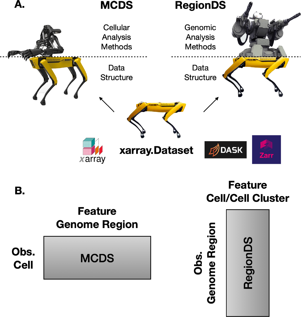
Fig. 5 A. The bases are the same and the methods are different. B. MCDS is cell-by-region matrix for cellular analysis; RegionDS is region-by-cell matrix for genomic analysis.¶

Input Files

Contents