Basic Cell Clustering Using 100Kb Bins
Contents
Basic Cell Clustering Using 100Kb Bins
Content
Here we go through the basic steps to perform cell clustering using genome non-overlapping 100Kb bins as features. We start from raw methylation base count data stored in MCDS format. This notebook can be used to quickly evaluate cell-type composition in a single-cell methylome dataset (e.g., the dataset from a single experiment).
Dataset used in this notebook
Adult (age P56) male mouse brain hippocampus (HIP) snmC-seq2 data from [Liu et al., 2021].
Input
MCDS files (contains chrom100k count matrix)
Cell metadata
Output
Cell-by-100kb-bin AnnData with embedding coordinates and cluster labels.
Import
import pandas as pd
import numpy as np
import scanpy as sc
import matplotlib.pyplot as plt

from ALLCools.mcds import MCDS
from ALLCools.clustering import tsne, significant_pc_test, log_scale
from ALLCools.plot import *
Parameters
# change this to the path to your metadata
metadata_path = '../../data/Brain/snmC-seq2/HIP.CellMetadata.csv.gz'

# Basic filtering parameters.
# These are suggesting values, cutoff maybe different for different tissue and sequencing depths.
# To determine each cutoff more appropriately, one need to plot the distribution of each metric.
mapping_rate_cutoff = 0.5
mapping_rate_col_name = 'MappingRate'  # Name may change
final_reads_cutoff = 500000
final_reads_col_name = 'FinalReads'  # Name may change
mccc_cutoff = 0.03
mccc_col_name = 'mCCCFrac'  # Name may change
mch_cutoff = 0.2
mch_col_name = 'mCHFrac'  # Name may change
mcg_cutoff = 0.5
mcg_col_name = 'mCGFrac'  # Name may change

# change this to the paths to your MCDS files,
# ALLCools.MCDS can handle multiple MCDS files automatically
mcds_path = '../../data/Brain/snmC-seq2/Liu2021Nature.mcds/'

# Dimension name used to do clustering
# This corresponding to AnnData .obs and .var
obs_dim = 'cell'  # observation
var_dim = 'chrom100k'  # feature

# feature cov cutoffs
min_cov = 500
max_cov = 3000

# Regions to remove during the clustering analysis
# change this to the path to ENCODE blacklist.
# The ENCODE blacklist can be downloaded from https://github.com/Boyle-Lab/Blacklist/
black_list_path = '../../data/genome/mm10-blacklist.v2.bed.gz'
black_list_fraction = 0.2
exclude_chromosome = ['chrM', 'chrY']

# load to memory or not
load = True

# HVF
mch_pattern = 'CHN'
mcg_pattern = 'CGN'
n_top_feature = 20000

# PC cutoff
pc_cutoff = 0.1

# KNN
knn = -1  # -1 means auto determine

# Leiden
resolution = 1
Load Cell Metadata
metadata = pd.read_csv(metadata_path, index_col=0)
print(f'Metadata of {metadata.shape[0]} cells')
metadata.head()
Metadata of 16985 cells
| AllcPath | mCCCFrac | mCGFrac | mCGFracAdj | mCHFrac | mCHFracAdj | FinalReads | InputReads | MappedReads | DissectionRegion | BamFilteringRate | MappingRate | Plate | Col384 | Row384 | FANSDate | Slice | Sample | |
|---|---|---|---|---|---|---|---|---|---|---|---|---|---|---|---|---|---|---|
| 10E_M_0 | /gale/raidix/rdx-4/mapping/10E/CEMBA190625-10E... | 0.008198 | 0.822633 | 0.821166 | 0.041640 | 0.033718 | 1626504.0 | 4407752 | 2892347.0 | 10E | 0.562347 | 0.656195 | CEMBA190625-10E-1 | 0 | 0 | 190625 | 10 | 10E_190625 |
| 10E_M_1 | /gale/raidix/rdx-4/mapping/10E/CEMBA190625-10E... | 0.006019 | 0.743035 | 0.741479 | 0.024127 | 0.018218 | 2009998.0 | 5524084 | 3657352.0 | 10E | 0.549577 | 0.662074 | CEMBA190625-10E-1 | 0 | 1 | 190625 | 10 | 10E_190625 |
| 10E_M_10 | /gale/raidix/rdx-4/mapping/10E/CEMBA190625-10E... | 0.006569 | 0.750172 | 0.748520 | 0.027665 | 0.021235 | 1383636.0 | 3455260 | 2172987.0 | 10E | 0.636744 | 0.628892 | CEMBA190625-10E-1 | 19 | 0 | 190625 | 10 | 10E_190625 |
| 10E_M_101 | /gale/raidix/rdx-4/mapping/10E/CEMBA190625-10E... | 0.006353 | 0.760898 | 0.759369 | 0.026547 | 0.020323 | 2474670.0 | 7245482 | 4778768.0 | 10E | 0.517847 | 0.659551 | CEMBA190625-10E-1 | 18 | 3 | 190625 | 10 | 10E_190625 |
| 10E_M_102 | /gale/raidix/rdx-4/mapping/10E/CEMBA190625-10E... | 0.005409 | 0.752980 | 0.751637 | 0.019497 | 0.014164 | 2430290.0 | 7004754 | 4609570.0 | 10E | 0.527227 | 0.658063 | CEMBA190625-10E-1 | 19 | 2 | 190625 | 10 | 10E_190625 |
Filter Cells
judge = (metadata[mapping_rate_col_name] > mapping_rate_cutoff) & \
        (metadata[final_reads_col_name] > final_reads_cutoff) & \
        (metadata[mccc_col_name] < mccc_cutoff) & \
        (metadata[mch_col_name] < mch_cutoff) & \
        (metadata[mcg_col_name] > mcg_cutoff)

metadata = metadata[judge].copy()
print(f'{metadata.shape[0]} cells passed filtering')
16985 cells passed filtering
# Save
# metadata.to_csv('Brain.CellMetadata.PassQC.csv.gz')
Load MCDS
mcds = MCDS.open(
    mcds_path,
    obs_dim='cell',
    var_dim='chrom100k',
    use_obs=metadata.index  # MCDS contains all cells, this will select cells that passed filtering
)
total_feature = mcds.get_index(var_dim).size
mcds
<xarray.MCDS>
Dimensions:              (cell: 16985, chrom100k: 27269, count_type: 2, mc_type: 2)
Coordinates:
  * cell                 (cell) <U10 '10E_M_207' '10E_M_338' ... '9J_M_2969'
  * chrom100k            (chrom100k) int64 0 1 2 3 4 ... 27265 27266 27267 27268
    chrom100k_bin_end    (chrom100k) int64 dask.array<chunksize=(27269,), meta=np.ndarray>
    chrom100k_bin_start  (chrom100k) int64 dask.array<chunksize=(27269,), meta=np.ndarray>
    chrom100k_chrom      (chrom100k) <U5 dask.array<chunksize=(27269,), meta=np.ndarray>
  * count_type           (count_type) <U3 'mc' 'cov'
  * mc_type              (mc_type) <U3 'CGN' 'CHN'
    strand_type          <U4 'both'
Data variables:
    chrom100k_da         (cell, chrom100k, mc_type, count_type) uint16 dask.array<chunksize=(3397, 2479, 2, 2), meta=np.ndarray>
Attributes:
    obs_dim:  cell
var_dim: chrom100k# you can add the cell metadata into MCDS
mcds.add_cell_metadata(metadata)
Filter Features
mcds.add_feature_cov_mean(var_dim=var_dim)
Feature chrom100k mean cov across cells added in MCDS.coords['chrom100k_cov_mean'].
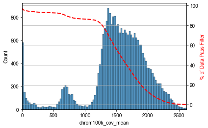
We saw three parts here with coverages from low to high, including:
Low coverage regions
chrX regions, because this dataset from male mouse brain
Other autosomal regions
# filter by coverage - based on the distribution above
mcds = mcds.filter_feature_by_cov_mean(
    min_cov=min_cov,  # minimum coverage
    max_cov=max_cov  # maximum coverage
)

# remove blacklist regions
mcds = mcds.remove_black_list_region(
    black_list_path=black_list_path,
    f=black_list_fraction  # Features having overlap > f with any black list region will be removed.
)

# remove chromosomes
mcds = mcds.remove_chromosome(exclude_chromosome)
Before cov mean filter: 27269 chrom100k
 After cov mean filter: 25242 chrom100k 92.6%
1189 chrom100k features removed due to overlapping (bedtools intersect -f 0.2) with black list regions.
20 chrom100k features in ['chrM', 'chrY'] removed.
Calculate Feature mC Fractions
mcds.add_mc_frac(
normalize_per_cell=True,  # after calculating mC frac, per cell normalize the matrix
    clip_norm_value=10  # clip outlier values above 10 to 10
)

# load only the mC fraction matrix into memory so following steps is faster
# Only load into memory when your memory size is enough to handle your dataset
if load and (mcds.get_index(obs_dim).size < 20000):
    mcds[f'{var_dim}_da_frac'].load()
/home/hanliu/miniconda3/envs/allcools_new/lib/python3.8/site-packages/dask/core.py:119: RuntimeWarning: invalid value encountered in true_divide
  return func(*(_execute_task(a, cache) for a in args))
The RuntimeWarning is expected (due to cov == 0). You can ignore it.
Select Highly Variable Features (HVF)
mCH HVF
mch_hvf = mcds.calculate_hvf_svr(var_dim=var_dim,
                                 mc_type=mch_pattern,
                                 n_top_feature=n_top_feature,
                                 plot=True)
Fitting SVR with gamma 0.0416, predicting feature dispersion using mc_frac_mean and cov_mean.
Total Feature Number:     24045
Highly Variable Feature:  20000 (83.2%)
mCG HVF
mcg_hvf = mcds.calculate_hvf_svr(var_dim=var_dim,
                                 mc_type=mcg_pattern,
                                 n_top_feature=n_top_feature,
                                 plot=True)
Fitting SVR with gamma 0.0416, predicting feature dispersion using mc_frac_mean and cov_mean.
Total Feature Number:     24045
Highly Variable Feature:  20000 (83.2%)
Get cell-by-feature mC fraction AnnData
mch_adata = mcds.get_adata(mc_type=mch_pattern,
                           var_dim=var_dim,
                           select_hvf=True)
mch_adata
AnnData object with n_obs × n_vars = 16985 × 20000
    obs: 'AllcPath', 'mCCCFrac', 'mCGFrac', 'mCGFracAdj', 'mCHFrac', 'mCHFracAdj', 'FinalReads', 'InputReads', 'MappedReads', 'DissectionRegion', 'BamFilteringRate', 'MappingRate', 'Plate', 'Col384', 'Row384', 'FANSDate', 'Slice', 'Sample'
    var: 'bin_end', 'bin_start', 'chrom', 'cov_mean', 'CHN_mean', 'CHN_dispersion', 'CHN_cov', 'CHN_score', 'CHN_feature_select', 'CGN_mean', 'CGN_dispersion', 'CGN_cov', 'CGN_score', 'CGN_feature_select'
mcg_adata = mcds.get_adata(mc_type=mcg_pattern,
                           var_dim=var_dim,
                           select_hvf=True)
mcg_adata
AnnData object with n_obs × n_vars = 16985 × 20000
    obs: 'AllcPath', 'mCCCFrac', 'mCGFrac', 'mCGFracAdj', 'mCHFrac', 'mCHFracAdj', 'FinalReads', 'InputReads', 'MappedReads', 'DissectionRegion', 'BamFilteringRate', 'MappingRate', 'Plate', 'Col384', 'Row384', 'FANSDate', 'Slice', 'Sample'
    var: 'bin_end', 'bin_start', 'chrom', 'cov_mean', 'CHN_mean', 'CHN_dispersion', 'CHN_cov', 'CHN_score', 'CHN_feature_select', 'CGN_mean', 'CGN_dispersion', 'CGN_cov', 'CGN_score', 'CGN_feature_select'
Scale
log_scale(mch_adata)
StandardScaler(with_mean=False)
log_scale(mcg_adata)
StandardScaler(with_mean=False)
PCA
mCH PCA
sc.tl.pca(mch_adata)
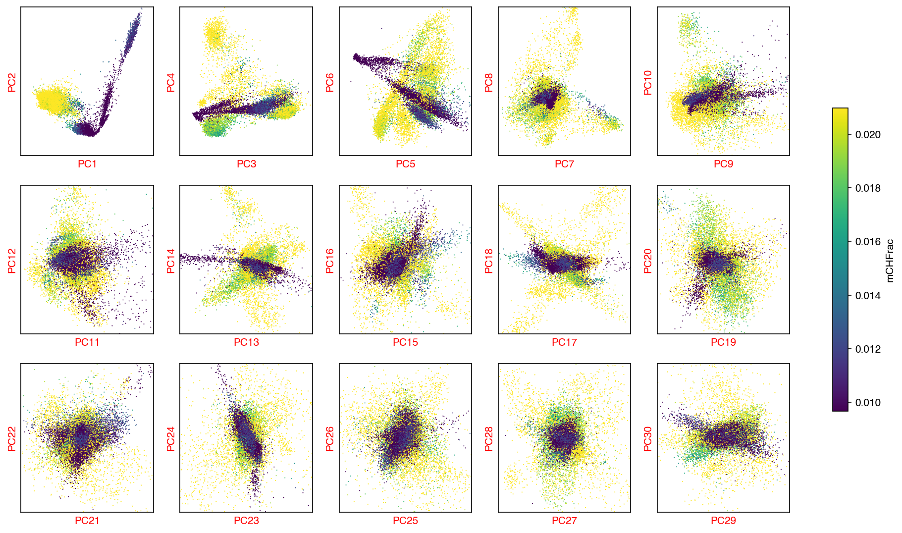
ch_n_components = significant_pc_test(mch_adata)
fig, axes = plot_decomp_scatters(mch_adata,
n_components=ch_n_components,
hue=mch_col_name,
hue_quantile=(0.25, 0.75),
nrows=3,
ncols=5)
47 components passed P cutoff of 0.1.
Changing adata.obsm['X_pca'] from shape (16985, 50) to (16985, 47)
Red axis labels are used PCs
mCG PCA
sc.tl.pca(mcg_adata)
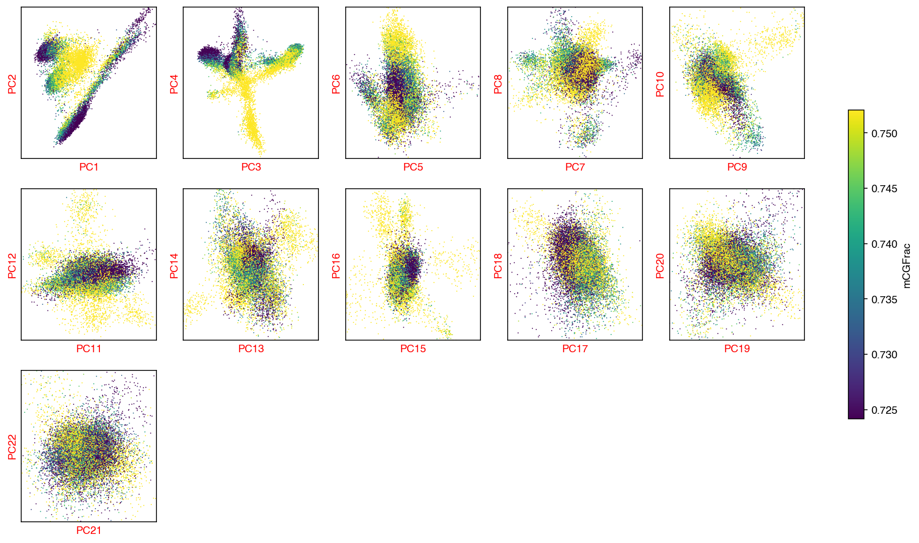
cg_n_components = significant_pc_test(mcg_adata)
fig, axes = plot_decomp_scatters(mcg_adata,
n_components=cg_n_components,
hue=mcg_col_name,
hue_quantile=(0.25, 0.75),
nrows=3,
ncols=5)
23 components passed P cutoff of 0.1.
Changing adata.obsm['X_pca'] from shape (16985, 50) to (16985, 23)
Red axis labels are used PCs
Concatenate PCs
ch_pcs = mch_adata.obsm['X_pca'][:, :ch_n_components]
cg_pcs = mcg_adata.obsm['X_pca'][:, :cg_n_components]

# scale the PCs so CH and CG PCs has the same total var
cg_pcs = cg_pcs / cg_pcs.std()
ch_pcs = ch_pcs / ch_pcs.std()

# total_pcs
total_pcs = np.hstack([ch_pcs, cg_pcs])

# make a copy of adata, add new pcs
# this is suboptimal, will change this when adata can combine layer and X in the future
adata = mch_adata.copy()
adata.obsm['X_pca'] = total_pcs
del adata.uns['pca']
del adata.varm['PCs']
Clustering
Calculate Nearest Neighbors
if knn == -1:
    knn = max(15, int(np.log2(adata.shape[0])*2))
sc.pp.neighbors(adata, n_neighbors=knn)
Leiden Clustering
sc.tl.leiden(adata, resolution=resolution)
Manifold learning
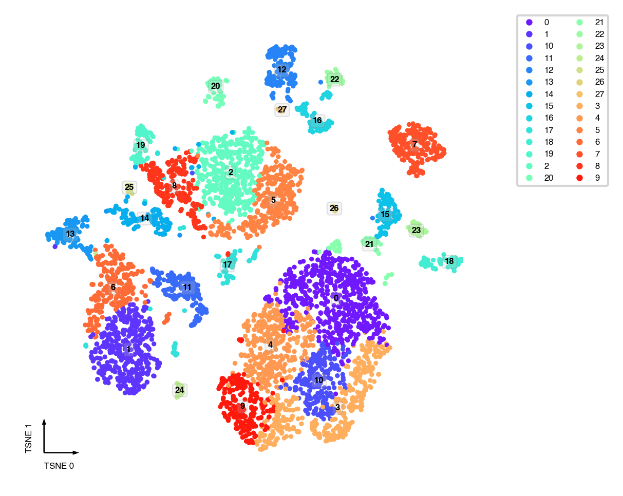
tSNE
tsne(adata,
     obsm='X_pca',
     metric='euclidean',
     exaggeration=-1,  # auto determined
     perplexity=30,
     n_jobs=-1)
fig, ax = plt.subplots(figsize=(4, 4), dpi=300)
_ = categorical_scatter(data=adata,
                        ax=ax,
                        coord_base='tsne',
                        hue='leiden',
                        text_anno='leiden',
                        show_legend=True)
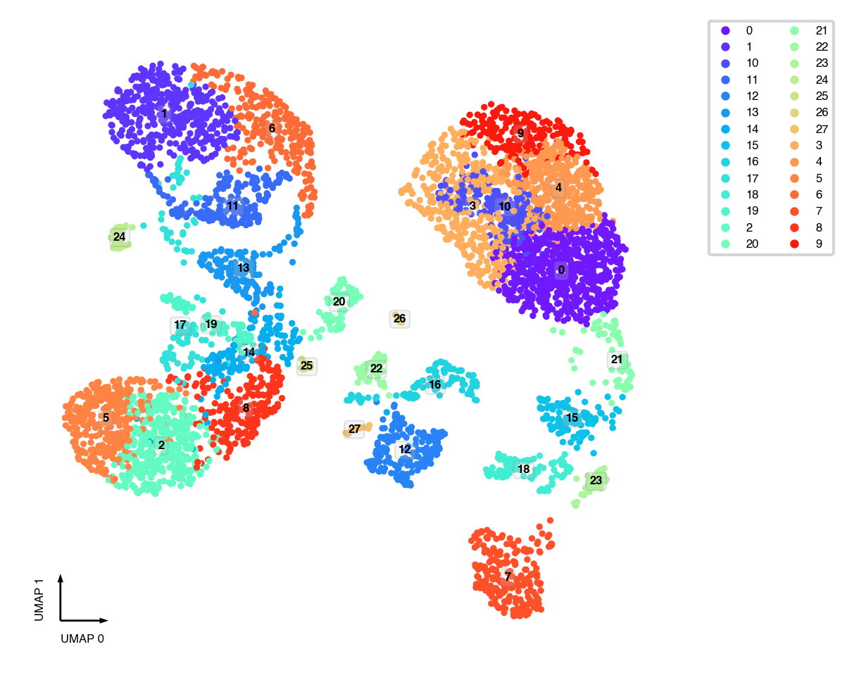
UMAP
sc.tl.umap(adata)
fig, ax = plt.subplots(figsize=(4, 4), dpi=300)
_ = categorical_scatter(data=adata,
                        ax=ax,
                        coord_base='umap',
                        hue='leiden',
                        text_anno='leiden',
                        show_legend=True)
Interactive plot
# in order to reduce the page size, I downsample the data here, you don't need to do this
interactive_scatter(data=adata,
                    hue='leiden',
                    coord_base='umap',
                    max_points=3000)
Save Results
adata.write_h5ad('Brain.chrom100k-clustering.h5ad')
adata
/home/hanliu/miniconda3/envs/allcools_new/lib/python3.8/site-packages/anndata/_core/anndata.py:1228: FutureWarning:

The `inplace` parameter in pandas.Categorical.reorder_categories is deprecated and will be removed in a future version. Reordering categories will always return a new Categorical object.

... storing 'DissectionRegion' as categorical
/home/hanliu/miniconda3/envs/allcools_new/lib/python3.8/site-packages/anndata/_core/anndata.py:1228: FutureWarning:

The `inplace` parameter in pandas.Categorical.reorder_categories is deprecated and will be removed in a future version. Reordering categories will always return a new Categorical object.

... storing 'Plate' as categorical
/home/hanliu/miniconda3/envs/allcools_new/lib/python3.8/site-packages/anndata/_core/anndata.py:1228: FutureWarning:

The `inplace` parameter in pandas.Categorical.reorder_categories is deprecated and will be removed in a future version. Reordering categories will always return a new Categorical object.

... storing 'Sample' as categorical
/home/hanliu/miniconda3/envs/allcools_new/lib/python3.8/site-packages/anndata/_core/anndata.py:1228: FutureWarning:

The `inplace` parameter in pandas.Categorical.reorder_categories is deprecated and will be removed in a future version. Reordering categories will always return a new Categorical object.

... storing 'chrom' as categorical
AnnData object with n_obs × n_vars = 16985 × 20000
    obs: 'AllcPath', 'mCCCFrac', 'mCGFrac', 'mCGFracAdj', 'mCHFrac', 'mCHFracAdj', 'FinalReads', 'InputReads', 'MappedReads', 'DissectionRegion', 'BamFilteringRate', 'MappingRate', 'Plate', 'Col384', 'Row384', 'FANSDate', 'Slice', 'Sample', 'leiden'
    var: 'bin_end', 'bin_start', 'chrom', 'cov_mean', 'CHN_mean', 'CHN_dispersion', 'CHN_cov', 'CHN_score', 'CHN_feature_select', 'CGN_mean', 'CGN_dispersion', 'CGN_cov', 'CGN_score', 'CGN_feature_select'
    uns: 'log', 'neighbors', 'leiden', 'umap'
    obsm: 'X_pca', 'X_tsne', 'X_umap'
    obsp: 'distances', 'connectivities'
adata.obs.to_csv('Brain.ClusteringResults.csv.gz')
adata.obs.head()
| AllcPath | mCCCFrac | mCGFrac | mCGFracAdj | mCHFrac | mCHFracAdj | FinalReads | InputReads | MappedReads | DissectionRegion | BamFilteringRate | MappingRate | Plate | Col384 | Row384 | FANSDate | Slice | Sample | leiden | |
|---|---|---|---|---|---|---|---|---|---|---|---|---|---|---|---|---|---|---|---|
| cell | |||||||||||||||||||
| 10E_M_207 | /gale/raidix/rdx-4/mapping/10E/CEMBA190625-10E... | 0.006059 | 0.791481 | 0.790210 | 0.024853 | 0.018908 | 1394119.0 | 3382862 | 2208361.0 | 10E | 0.631291 | 0.652808 | CEMBA190625-10E-2 | 20 | 4 | 190625 | 10 | 10E_190625 | 14 |
| 10E_M_338 | /gale/raidix/rdx-4/mapping/10E/CEMBA190625-10E... | 0.005151 | 0.738883 | 0.737531 | 0.017620 | 0.012533 | 1623613.0 | 3930932 | 2616811.0 | 10E | 0.620455 | 0.665697 | CEMBA190625-10E-1 | 9 | 6 | 190625 | 10 | 10E_190625 | 14 |
| 10E_M_410 | /gale/raidix/rdx-4/mapping/10E/CEMBA190625-10E... | 0.005322 | 0.741459 | 0.740076 | 0.017949 | 0.012695 | 1698314.0 | 4325806 | 2883026.0 | 10E | 0.589073 | 0.666471 | CEMBA190625-10E-1 | 3 | 9 | 190625 | 10 | 10E_190625 | 8 |
| 10E_M_426 | /gale/raidix/rdx-4/mapping/10E/CEMBA190625-10E... | 0.005194 | 0.729766 | 0.728355 | 0.017188 | 0.012057 | 1830508.0 | 4893582 | 3245794.0 | 10E | 0.563963 | 0.663276 | CEMBA190625-10E-1 | 7 | 9 | 190625 | 10 | 10E_190625 | 14 |
| 10E_M_431 | /gale/raidix/rdx-4/mapping/10E/CEMBA190625-10E... | 0.006075 | 0.756491 | 0.755003 | 0.023721 | 0.017754 | 1585419.0 | 4273210 | 2838002.0 | 10E | 0.558639 | 0.664138 | CEMBA190625-10E-1 | 8 | 8 | 190625 | 10 | 10E_190625 | 14 |
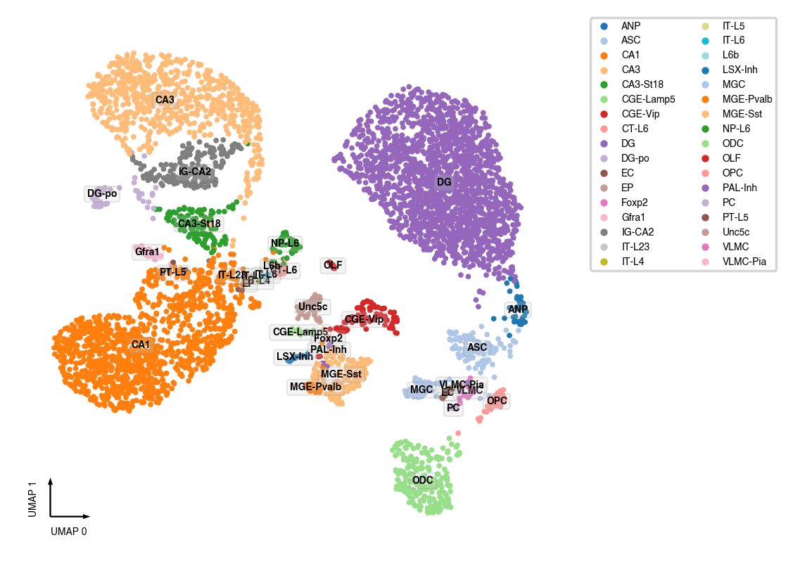
Sanity test
This test dataset come from [Liu et al., 2021], so we already annotated the cell types. For new datasets, see following notebooks about identifying cluster markers and annotate clusters
try:
    cell_anno = pd.read_csv('../../data/Brain/snmC-seq2/HIP.Annotated.CellMetadata.csv.gz', index_col=0)
    fig, ax = plt.subplots(figsize=(4, 4), dpi=250)
    adata.obs['CellTypeAnno'] = cell_anno['MajorType']
    adata.obs['CellTypeAnno'].fillna('nan', inplace=True)
    _ = categorical_scatter(data=adata,
                            ax=ax,
                            coord_base='umap',
                            hue='CellTypeAnno',
                            text_anno='CellTypeAnno',
                            palette='tab20',
                            show_legend=True)
except BaseException:
    pass