.ipynb .pdf

repository open issue suggest edit

Contents

DMR-Gene Correlation

Calculate the partial correlation between DMR and Genes using clusters/samples as features.

Import

import seaborn as sns
import matplotlib.pyplot as plt
from ALLCools.mcds import RegionDS
from ALLCools.mcds.correlation import region_correlation, get_corr_table

Load Data

# DMR data
dmr = RegionDS.open('../RegionDS/test_HIP/')

# gene data
gene = RegionDS.open('test_HIP_Cluster/', region_dim='geneslop2k')

Using dmr as region_dim

# global mC fractions, calculated from cell level MCDS by sum up cluster and genome base calls
sample_mch = gene.get_coords('sample_CHN')
sample_mcg = gene.get_coords('sample_CGN')

DMR Input

A 2-D sample-by-DMR DataArray, values are mCG fractions

data_a = dmr['dmr_da_frac'].transpose('sample', 'dmr')
data_a

<xarray.DataArray 'dmr_da_frac' (sample: 20, dmr: 131)>
array([[0.538462, 0.816129, 0.70068 , ..., 0.144186, 0.340136, 0.292444],
       [0.717949, 0.97006 , 0.922078, ..., 0.03    , 0.142259, 0.249802],
       [0.717949, 0.974227, 0.886179, ..., 0.011628, 0.085575, 0.196755],
       ...,
       [0.888889, 0.670588, 0.038462, ..., 0.55    , 0.25974 , 0.621951],
       [0.857143, 0.727823, 0.666667, ..., 0.295455, 0.562387, 0.544554],
       [0.777778, 0.780822, 0.5625  , ..., 0.0625  , 0.297297, 0.292553]],
      dtype=float32)
Coordinates:
  * dmr         (dmr) <U9 'chr1-0' 'chr1-1' 'chr1-2' ... 'chr19-121' 'chr19-122'
    dmr_chrom   (dmr) <U5 'chr1' 'chr1' 'chr1' ... 'chr19' 'chr19' 'chr19'
    dmr_end     (dmr) int64 10002172 10003542 10003967 ... 5099203 5099952
    dmr_length  (dmr) int64 2 305 54 2 2 2 10 ... 589 924 632 842 195 399 335
    dmr_ndms    (dmr) int64 1 7 2 1 1 1 2 13 3 2 1 ... 2 1 2 7 13 19 8 8 3 6 13
    dmr_start   (dmr) int64 10002170 10003237 10003913 ... 5098804 5099617
  * sample      (sample) <U18 'snm3C_ASC' 'snm3C_CA1' ... 'snmC_ODC' 'snmC_OPC'

xarray.DataArray

'dmr_da_frac'

• sample: 20
• dmr: 131

• 0.5385 0.8161 0.7007 0.8 0.3846 ... 0.4409 0.5833 0.0625 0.2973 0.2926

  array([[0.538462, 0.816129, 0.70068 , ..., 0.144186, 0.340136, 0.292444],
         [0.717949, 0.97006 , 0.922078, ..., 0.03    , 0.142259, 0.249802],
         [0.717949, 0.974227, 0.886179, ..., 0.011628, 0.085575, 0.196755],
         ...,
         [0.888889, 0.670588, 0.038462, ..., 0.55    , 0.25974 , 0.621951],
         [0.857143, 0.727823, 0.666667, ..., 0.295455, 0.562387, 0.544554],
         [0.777778, 0.780822, 0.5625  , ..., 0.0625  , 0.297297, 0.292553]],
        dtype=float32)

• Coordinates: (7)
  • dmr
    (dmr)
    <U9
    'chr1-0' 'chr1-1' ... 'chr19-122'

    array(['chr1-0', 'chr1-1', 'chr1-2', 'chr1-3', 'chr1-4', 'chr1-5', 'chr1-6',
           'chr1-7', 'chr19-0', 'chr19-1', 'chr19-2', 'chr19-3', 'chr19-4',
           'chr19-5', 'chr19-6', 'chr19-7', 'chr19-8', 'chr19-9', 'chr19-10',
           'chr19-11', 'chr19-12', 'chr19-13', 'chr19-14', 'chr19-15', 'chr19-16',
           'chr19-17', 'chr19-18', 'chr19-19', 'chr19-20', 'chr19-21', 'chr19-22',
           'chr19-23', 'chr19-24', 'chr19-25', 'chr19-26', 'chr19-27', 'chr19-28',
           'chr19-29', 'chr19-30', 'chr19-31', 'chr19-32', 'chr19-33', 'chr19-34',
           'chr19-35', 'chr19-36', 'chr19-37', 'chr19-38', 'chr19-39', 'chr19-40',
           'chr19-41', 'chr19-42', 'chr19-43', 'chr19-44', 'chr19-45', 'chr19-46',
           'chr19-47', 'chr19-48', 'chr19-49', 'chr19-50', 'chr19-51', 'chr19-52',
           'chr19-53', 'chr19-54', 'chr19-55', 'chr19-56', 'chr19-57', 'chr19-58',
           'chr19-59', 'chr19-60', 'chr19-61', 'chr19-62', 'chr19-63', 'chr19-64',
           'chr19-65', 'chr19-66', 'chr19-67', 'chr19-68', 'chr19-69', 'chr19-70',
           'chr19-71', 'chr19-72', 'chr19-73', 'chr19-74', 'chr19-75', 'chr19-76',
           'chr19-77', 'chr19-78', 'chr19-79', 'chr19-80', 'chr19-81', 'chr19-82',
           'chr19-83', 'chr19-84', 'chr19-85', 'chr19-86', 'chr19-87', 'chr19-88',
           'chr19-89', 'chr19-90', 'chr19-91', 'chr19-92', 'chr19-93', 'chr19-94',
           'chr19-95', 'chr19-96', 'chr19-97', 'chr19-98', 'chr19-99', 'chr19-100',
           'chr19-101', 'chr19-102', 'chr19-103', 'chr19-104', 'chr19-105',
           'chr19-106', 'chr19-107', 'chr19-108', 'chr19-109', 'chr19-110',
           'chr19-111', 'chr19-112', 'chr19-113', 'chr19-114', 'chr19-115',
           'chr19-116', 'chr19-117', 'chr19-118', 'chr19-119', 'chr19-120',
           'chr19-121', 'chr19-122'], dtype='<U9')

  • dmr_chrom
    (dmr)
    <U5
    'chr1' 'chr1' ... 'chr19' 'chr19'

    array(['chr1', 'chr1', 'chr1', 'chr1', 'chr1', 'chr1', 'chr1', 'chr1',
           'chr19', 'chr19', 'chr19', 'chr19', 'chr19', 'chr19', 'chr19',
           'chr19', 'chr19', 'chr19', 'chr19', 'chr19', 'chr19', 'chr19',
           'chr19', 'chr19', 'chr19', 'chr19', 'chr19', 'chr19', 'chr19',
           'chr19', 'chr19', 'chr19', 'chr19', 'chr19', 'chr19', 'chr19',
           'chr19', 'chr19', 'chr19', 'chr19', 'chr19', 'chr19', 'chr19',
           'chr19', 'chr19', 'chr19', 'chr19', 'chr19', 'chr19', 'chr19',
           'chr19', 'chr19', 'chr19', 'chr19', 'chr19', 'chr19', 'chr19',
           'chr19', 'chr19', 'chr19', 'chr19', 'chr19', 'chr19', 'chr19',
           'chr19', 'chr19', 'chr19', 'chr19', 'chr19', 'chr19', 'chr19',
           'chr19', 'chr19', 'chr19', 'chr19', 'chr19', 'chr19', 'chr19',
           'chr19', 'chr19', 'chr19', 'chr19', 'chr19', 'chr19', 'chr19',
           'chr19', 'chr19', 'chr19', 'chr19', 'chr19', 'chr19', 'chr19',
           'chr19', 'chr19', 'chr19', 'chr19', 'chr19', 'chr19', 'chr19',
           'chr19', 'chr19', 'chr19', 'chr19', 'chr19', 'chr19', 'chr19',
           'chr19', 'chr19', 'chr19', 'chr19', 'chr19', 'chr19', 'chr19',
           'chr19', 'chr19', 'chr19', 'chr19', 'chr19', 'chr19', 'chr19',
           'chr19', 'chr19', 'chr19', 'chr19', 'chr19', 'chr19', 'chr19',
           'chr19', 'chr19', 'chr19', 'chr19'], dtype='<U5')

  • dmr_end
    (dmr)
    int64
    10002172 10003542 ... 5099952

    array([10002172, 10003542, 10003967, 10005479, 10007099, 10007758,
           10008889, 10009927,  5000194,  5000343,  5000715,  5001506,
            5001549,  5003862,  5004785,  5005319,  5005816,  5006789,
            5008015,  5008084,  5008130,  5008805,  5010091,  5011268,
            5011724,  5011926,  5012429,  5012955,  5013312,  5013603,
            5014250,  5014562,  5014921,  5015099,  5016145,  5016791,
            5017134,  5017656,  5018165,  5018294,  5019014,  5019656,
            5020498,  5021894,  5022034,  5022299,  5023452,  5025645,
            5026013,  5026581,  5028070,  5029223,  5029469,  5029930,
            5031623,  5031970,  5032343,  5033665,  5035273,  5036180,
            5036656,  5037800,  5040294,  5040872,  5042216,  5042541,
            5043207,  5043818,  5045206,  5046083,  5046469,  5047139,
            5050164,  5051764,  5054110,  5055419,  5056089,  5056189,
            5056309,  5056642,  5057152,  5057233,  5059120,  5059541,
            5060286,  5060636,  5061033,  5061586,  5062181,  5063226,
            5064727,  5065461,  5065765,  5066074,  5066405,  5067916,
            5069149,  5070132,  5071656,  5071800,  5073983,  5074921,
            5076037,  5076379,  5077207,  5078490,  5078805,  5080040,
            5080229,  5081032,  5081240,  5081796,  5082893,  5083285,
            5083313,  5084274,  5084686,  5086323,  5087151,  5087539,
            5089466,  5089734,  5090283,  5091820,  5092737,  5094022,
            5095601,  5097380,  5097870,  5099203,  5099952])

  • dmr_length
    (dmr)
    int64
    2 305 54 2 2 ... 842 195 399 335

    array([   2,  305,   54,    2,    2,    2,   10,  440,  171,   12,    2,
              2,   22,  504,  128,  146,  201,    2,    2,    2,    2,  182,
              2,  246,    2,    2,  101,  343,   49,  183,    2,   88,    2,
              2,   89,  385,    8,    2,    2,    2,  144,    2,    2,  821,
              2,    2,  306,  913,    2,   71,   91,   22,   21,  149,    2,
              2,    2,    2,    2,   57,   76,    2,  532,  552,  211,    2,
            243,    2,    2,  322,   63,    2, 2314, 1029, 2090,    2,   58,
              2,    2,    2,  253,    2, 1191,    2,  478,    2,  127,   42,
             43,    2,    2,  482,   14,    2,    2,  773,  760,    2,  661,
            126,  345,  687,  366,    2,  469,  866,    2,    2,   59,  315,
              2,  368, 1053,  367,    2,  186,    2,  391,  158,  323,   31,
              2,  138,  434,  589,  924,  632,  842,  195,  399,  335])

  • dmr_ndms
    (dmr)
    int64
    1 7 2 1 1 1 2 ... 13 19 8 8 3 6 13

    array([ 1,  7,  2,  1,  1,  1,  2, 13,  3,  2,  1,  1,  2,  5,  2,  3,  2,
            1,  1,  1,  1,  4,  1,  2,  1,  1,  3,  6,  4,  3,  1,  4,  1,  1,
            3,  6,  3,  1,  1,  1,  4,  1,  1,  8,  1,  1,  9, 14,  1,  4,  3,
            2,  2,  2,  1,  1,  1,  1,  1,  2,  2,  1, 17, 11,  3,  1,  5,  1,
            1,  9,  4,  1, 33, 27, 57,  1,  2,  1,  1,  1,  4,  1, 19,  1,  7,
            1,  2,  2,  2,  1,  1,  7,  3,  1,  1, 15, 29,  1, 20,  4,  8, 13,
            4,  1,  5, 15,  1,  1,  4,  6,  1, 10, 47,  9,  1,  2,  1,  3,  5,
            8,  2,  1,  2,  7, 13, 19,  8,  8,  3,  6, 13])

  • dmr_start
    (dmr)
    int64
    10002170 10003237 ... 5099617

    array([10002170, 10003237, 10003913, 10005477, 10007097, 10007756,
           10008879, 10009487,  5000023,  5000331,  5000713,  5001504,
            5001527,  5003358,  5004657,  5005173,  5005615,  5006787,
            5008013,  5008082,  5008128,  5008623,  5010089,  5011022,
            5011722,  5011924,  5012328,  5012612,  5013263,  5013420,
            5014248,  5014474,  5014919,  5015097,  5016056,  5016406,
            5017126,  5017654,  5018163,  5018292,  5018870,  5019654,
            5020496,  5021073,  5022032,  5022297,  5023146,  5024732,
            5026011,  5026510,  5027979,  5029201,  5029448,  5029781,
            5031621,  5031968,  5032341,  5033663,  5035271,  5036123,
            5036580,  5037798,  5039762,  5040320,  5042005,  5042539,
            5042964,  5043816,  5045204,  5045761,  5046406,  5047137,
            5047850,  5050735,  5052020,  5055417,  5056031,  5056187,
            5056307,  5056640,  5056899,  5057231,  5057929,  5059539,
            5059808,  5060634,  5060906,  5061544,  5062138,  5063224,
            5064725,  5064979,  5065751,  5066072,  5066403,  5067143,
            5068389,  5070130,  5070995,  5071674,  5073638,  5074234,
            5075671,  5076377,  5076738,  5077624,  5078803,  5080038,
            5080170,  5080717,  5081238,  5081428,  5081840,  5082918,
            5083311,  5084088,  5084684,  5085932,  5086993,  5087216,
            5089435,  5089732,  5090145,  5091386,  5092148,  5093098,
            5094969,  5096538,  5097675,  5098804,  5099617])

  • sample
    (sample)
    <U18
    'snm3C_ASC' ... 'snmC_OPC'

    array(['snm3C_ASC', 'snm3C_CA1', 'snm3C_CA23', 'snm3C_CGE-VipLamp5',
           'snm3C_DG', 'snm3C_MGC', 'snm3C_MGE-PvSst', 'snm3C_NonN', 'snm3C_ODC',
           'snm3C_OPC', 'snmC_ASC', 'snmC_CA1', 'snmC_CA23', 'snmC_CGE-VipLamp5',
           'snmC_DG', 'snmC_MGC', 'snmC_MGE-PvSst', 'snmC_NonN', 'snmC_ODC',
           'snmC_OPC'], dtype='<U18')

• Attributes: (0)

Gene Input

A 2-D sample-by-gene DataArray, values are cluster-normalized mCH fractions

data_b = gene.sel(
    mc_type='CHN',
    sample=data_a.get_index('sample'))['geneslop2k_da_frac'].transpose(
        'sample', 'geneslop2k')
data_b

<xarray.DataArray 'geneslop2k_da_frac' (sample: 20, geneslop2k: 55487)>
[1109740 values with dtype=float64]
Coordinates:
    mc_type           <U3 'CHN'
  * sample            (sample) object 'snm3C_ASC' 'snm3C_CA1' ... 'snmC_OPC'
    sample_CGN        (sample) float64 0.7203 0.7387 0.7422 ... 0.7434 0.7196
    sample_CHN        (sample) float64 0.007835 0.02362 ... 0.01121 0.005743
    strand_type       <U4 'both'
  * geneslop2k        (geneslop2k) object 'ENSMUSG00000102693.1' ... 'ENSMUSG...
    geneslop2k_chrom  (geneslop2k) object 'chr1' 'chr1' 'chr1' ... 'chrM' 'chrM'
    geneslop2k_end    (geneslop2k) int64 3076321 3104124 3673497 ... 16299 16299
    geneslop2k_start  (geneslop2k) int64 3071252 3100015 3203900 ... 13288 13355

xarray.DataArray

'geneslop2k_da_frac'

• sample: 20
• geneslop2k: 55487

• ...

  [1109740 values with dtype=float64]

• Coordinates: (9)
  • mc_type
    ()
    <U3
    'CHN'

    array('CHN', dtype='<U3')

  • sample
    (sample)
    object
    'snm3C_ASC' ... 'snmC_OPC'

    array(['snm3C_ASC', 'snm3C_CA1', 'snm3C_CA23', 'snm3C_CGE-VipLamp5',
           'snm3C_DG', 'snm3C_MGC', 'snm3C_MGE-PvSst', 'snm3C_NonN', 'snm3C_ODC',
           'snm3C_OPC', 'snmC_ASC', 'snmC_CA1', 'snmC_CA23', 'snmC_CGE-VipLamp5',
           'snmC_DG', 'snmC_MGC', 'snmC_MGE-PvSst', 'snmC_NonN', 'snmC_ODC',
           'snmC_OPC'], dtype=object)

  • sample_CGN
    (sample)
    float64
    0.7203 0.7387 ... 0.7434 0.7196

    array([0.72027702, 0.7386765 , 0.74223235, 0.78137746, 0.70998683,
           0.69529767, 0.79745986, 0.6957201 , 0.72761756, 0.70625517,
           0.73871943, 0.74009099, 0.75324386, 0.80065615, 0.72773628,
           0.71349106, 0.8149437 , 0.70807914, 0.74336865, 0.71960449])

  • sample_CHN
    (sample)
    float64
    0.007835 0.02362 ... 0.005743

    array([0.00783526, 0.02362182, 0.02493468, 0.02857215, 0.0106706 ,
           0.00696775, 0.03594073, 0.00793199, 0.01268308, 0.00754718,
           0.00681991, 0.01997363, 0.02210814, 0.02925379, 0.00979016,
           0.00561416, 0.03664812, 0.00748145, 0.01121077, 0.00574326])

  • strand_type
    ()
    <U4
    'both'

    array('both', dtype='<U4')

  • geneslop2k
    (geneslop2k)
    object
    'ENSMUSG00000102693.1' ... 'ENSM...

    array(['ENSMUSG00000102693.1', 'ENSMUSG00000064842.1', 'ENSMUSG00000051951.5',
           ..., 'ENSMUSG00000064370.1', 'ENSMUSG00000064371.1',
           'ENSMUSG00000064372.1'], dtype=object)

  • geneslop2k_chrom
    (geneslop2k)
    object
    'chr1' 'chr1' ... 'chrM' 'chrM'

    array(['chr1', 'chr1', 'chr1', ..., 'chrM', 'chrM', 'chrM'], dtype=object)

  • geneslop2k_end
    (geneslop2k)
    int64
    3076321 3104124 ... 16299 16299

    array([3076321, 3104124, 3673497, ...,   16299,   16299,   16299])

  • geneslop2k_start
    (geneslop2k)
    int64
    3071252 3100015 ... 13288 13355

    array([3071252, 3100015, 3203900, ...,   12144,   13288,   13355])

• Attributes: (0)

Calculate correlations between DMR and genes

true_results, null_results = region_correlation(data_a,
                                                data_b,
                                                sample_mch,
                                                sample_mcg,
                                                method='pearson',
                                                max_dist=1000000,
                                                cpu=40,
                                                null='sample',
                                                null_n=100000)

Using dmr as region_dim
Using dmr_start and dmr_end to calculate pos
Using geneslop2k as region_dim
Using geneslop2k_start and geneslop2k_end to calculate pos
Calculating chr1
Calculating chr19

true_results.X.data.size, null_results.size

(19100, 19100)

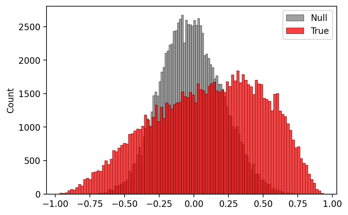
Plot correlation distribution

import numpy as np

fig, ax = plt.subplots(dpi=200)
sns.histplot(ax=ax,
             data=np.random.choice(null_results, 100000),
             label='Null',
             bins=100,
             color='grey')
sns.histplot(ax=ax,
             data=np.random.choice(true_results.X.data, 100000),
             label='True',
             bins=100,
             color='red')
ax.legend()

<matplotlib.legend.Legend at 0x7f5ce2c67b80>

findfont: Font family ['sans-serif'] not found. Falling back to DejaVu Sans.
findfont: Generic family 'sans-serif' not found because none of the following families were found: Helvetica

Get Significantly Correlated Pairs

corr_table = get_corr_table(true_results,
                            null_results,
                            region_dim_a=data_a.dims[1],
                            region_dim_b=data_b.dims[1],
                            direction='+',
                            alpha=0.03)

corr_table['pair_distance'] = corr_table['dmr_pos'] - corr_table['geneslop2k_pos']

corr_table

Correlation cutoff corr > 0.5499999999999998
2855 correlation pairs selected.

	dmr	geneslop2k	corr	dmr_pos	geneslop2k_pos	pair_distance
0	chr1-0	ENSMUSG00000025916.10	0.688226	10002171	9988879	13292
1	chr1-2	ENSMUSG00000102871.1	0.653428	10003940	9288550	715390
2	chr1-3	ENSMUSG00000067851.11	0.602079	10005478	10185119	-179641
3	chr1-3	ENSMUSG00000098234.7	0.560595	10005478	9943037	62441
4	chr1-3	ENSMUSG00000045210.8	0.701606	10005478	9733501	271977
...	...	...	...	...	...	...
2850	chr19-122	ENSMUSG00000024835.15	0.678979	5099784	4151326	948458
2851	chr19-122	ENSMUSG00000044724.9	0.811770	5099784	4142762	957022
2852	chr19-122	ENSMUSG00000024842.8	0.749665	5099784	4139727	960057
2853	chr19-122	ENSMUSG00000024845.17	0.655735	5099784	4129119	970665
2854	chr19-122	ENSMUSG00000024851.14	0.652242	5099784	4106980	992804

2855 rows × 6 columns

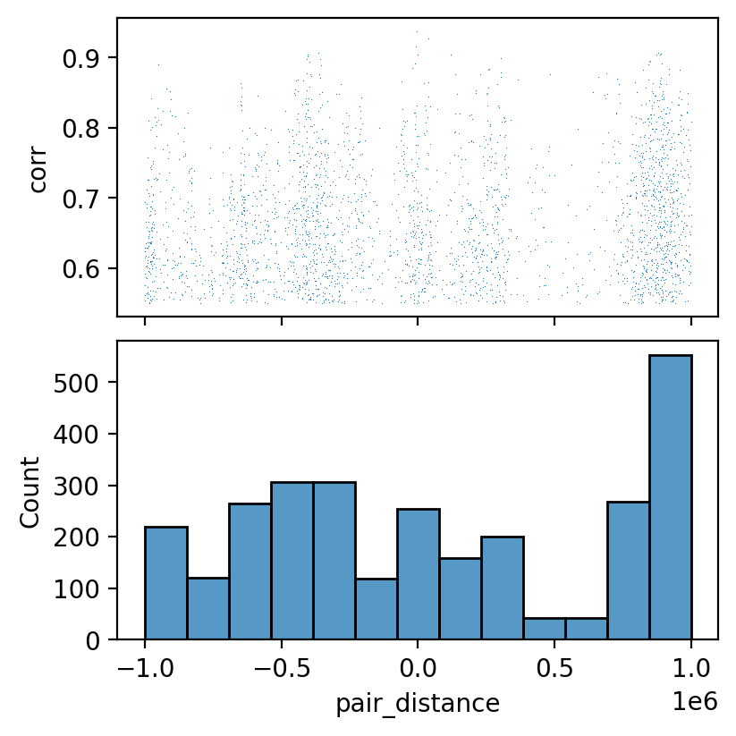
Plot distance and correlation distribution

fig, axes = plt.subplots(figsize=(4, 4), nrows=2, dpi=200, constrained_layout=True, sharex=True)

ax = axes[0]
sns.scatterplot(ax=ax,
                data=corr_table,
                x='pair_distance',
                y='corr',
                s=0.2,
                linewidth=0)
ax = axes[1]
sns.histplot(corr_table['pair_distance'], ax=ax)

<AxesSubplot:xlabel='pair_distance', ylabel='Count'>

previous

Prepare Cluster-by-Gene mC Profile

next

REPTILE