Basic Cell Clustering Using mCG-5Kb Bins¶

Content¶

Here we go through the basic steps to perform cell clustering using genome non-overlapping 5Kb bins as features. We start from hypo-methylation probability data stored in MCDS (quantified by the hypo- or hyper-methylation score option, see allcools generate-dataset). This notebook can be used to quickly evaluate cell-type composition in a single-cell methylome dataset (e.g., the dataset from a single experiment). Comparing with the 100Kb bins clustering process, this clustering process is more suitable for samples with low mCH fraction (many non-brain tissues) and narrow methylation diversity (so smaller feature works better).

Dataset used in this notebook¶

Adult (age P56) male mouse brain pituitary (PIT) snmC-seq2 data from [Ruf-Zamojski et al., 2021].

Input¶

MCDS with chrom5k hypo-score matrix
Cell metadata

Output¶

Cell-by-5kb-bin AnnData (sparse matrix) with embedding coordinates and cluster labels.

Import¶

import numpy as np
import pandas as pd
import matplotlib.pyplot as plt
import scanpy as sc
from ALLCools.mcds import MCDS
from ALLCools.clustering import tsne, significant_pc_test, filter_regions, lsi, binarize_matrix
from ALLCools.plot import *

Parameters¶

metadata_path = '../../data/PIT/PIT.CellMetadata.csv.gz'
mcds_path = '../../data/PIT/RufZamojski2021NC.mcds'

# Basic filtering parameters
mapping_rate_cutoff = 0.5
mapping_rate_col_name = 'MappingRate'  # Name may change
final_reads_cutoff = 500000
final_reads_col_name = 'FinalmCReads'  # Name may change
mccc_cutoff = 0.03
mccc_col_name = 'mCCCFrac'  # Name may change
mch_cutoff = 0.2
mch_col_name = 'mCHFrac'  # Name may change
mcg_cutoff = 0.5
mcg_col_name = 'mCGFrac'  # Name may change

# PC cutoff
pc_cutoff = 0.1

# KNN
knn = -1  # -1 means auto determine

# Leiden
resolution = 1

Load Cell Metadata¶

metadata = pd.read_csv(metadata_path, index_col=0)
print(f'Metadata of {metadata.shape[0]} cells')
metadata.head()

Metadata of 2756 cells

	CellInputReadPairs	MappingRate	FinalmCReads	mCCCFrac	mCGFrac	mCHFrac	Plate	Col384	Row384	CellTypeAnno
index
PIT_P1-PIT_P2-A1-AD001	1858622.0	0.685139	1612023.0	0.003644	0.679811	0.005782	PIT_P1	0	0	Outlier
PIT_P1-PIT_P2-A1-AD004	1599190.0	0.686342	1367004.0	0.004046	0.746012	0.008154	PIT_P1	1	0	Gonadotropes
PIT_P1-PIT_P2-A1-AD006	1932242.0	0.669654	1580990.0	0.003958	0.683584	0.005689	PIT_P1	1	1	Somatotropes
PIT_P1-PIT_P2-A1-AD007	1588505.0	0.664612	1292770.0	0.003622	0.735217	0.005460	PIT_P2	0	0	Rbpms+
PIT_P1-PIT_P2-A1-AD010	1738409.0	0.703835	1539676.0	0.003769	0.744640	0.006679	PIT_P2	1	0	Rbpms+

Filter Cells¶

judge = (metadata[mapping_rate_col_name] > mapping_rate_cutoff) & \
        (metadata[final_reads_col_name] > final_reads_cutoff) & \
        (metadata[mccc_col_name] < mccc_cutoff) & \
        (metadata[mch_col_name] < mch_cutoff) & \
        (metadata[mcg_col_name] > mcg_cutoff)

metadata = metadata[judge].copy()
# cell metadata for this example is filtered already
print(f'{metadata.shape[0]} cells passed filtering')

2756 cells passed filtering

Load hypo-methylation score matrix from MCDS¶

mcds = MCDS.open(mcds_path, var_dim='chrom5k')

mcds.add_cell_metadata(metadata)

mcds = mcds.remove_black_list_region(black_list_path='../../data/genome/mm10-blacklist.v2.bed.gz')

49908 chrom5k features removed due to overlapping (bedtools intersect -f 0.2) with black list regions.

mcad = mcds.get_score_adata(mc_type='CGN', quant_type='hypo-score')

mcad

AnnData object with n_obs × n_vars = 2756 × 495206
    obs: 'CellInputReadPairs', 'MappingRate', 'FinalmCReads', 'mCCCFrac', 'mCGFrac', 'mCHFrac', 'Plate', 'Col384', 'Row384', 'CellTypeAnno'
    var: 'chrom', 'end', 'start'

Binarize¶

binarize_matrix(mcad, cutoff=0.95)

Filter Features¶

filter_regions(mcad)

Filter out 206777 regions with # of non-zero cells <= 13

array([False, False, False, ...,  True,  True,  True])

mcad

AnnData object with n_obs × n_vars = 2756 × 288429
    obs: 'CellInputReadPairs', 'MappingRate', 'FinalmCReads', 'mCCCFrac', 'mCGFrac', 'mCHFrac', 'Plate', 'Col384', 'Row384', 'CellTypeAnno'
    var: 'chrom', 'end', 'start'

TF-IDF Transform and Dimension Reduction¶

# by default we save the results in adata.obsm['X_pca'] which is the scanpy defaults in many following functions
# But this matrix is not calculated by PCA
lsi(mcad, algorithm='arpack', obsm='X_pca')

TruncatedSVD(algorithm='arpack', n_components=100, random_state=0)

# choose significant components
significant_pc_test(mcad, p_cutoff=pc_cutoff, update=True)

13 components passed P cutoff of 0.1.
Changing adata.obsm['X_pca'] from shape (2756, 100) to (2756, 13)

Clustering¶

Calculate Nearest Neighbors¶

if knn == -1:
    knn = max(15, int(np.log2(mcad.shape[0])*2))
sc.pp.neighbors(mcad, n_neighbors=knn)

Leiden Clustering¶

sc.tl.leiden(mcad, resolution=resolution)

Manifold learning¶

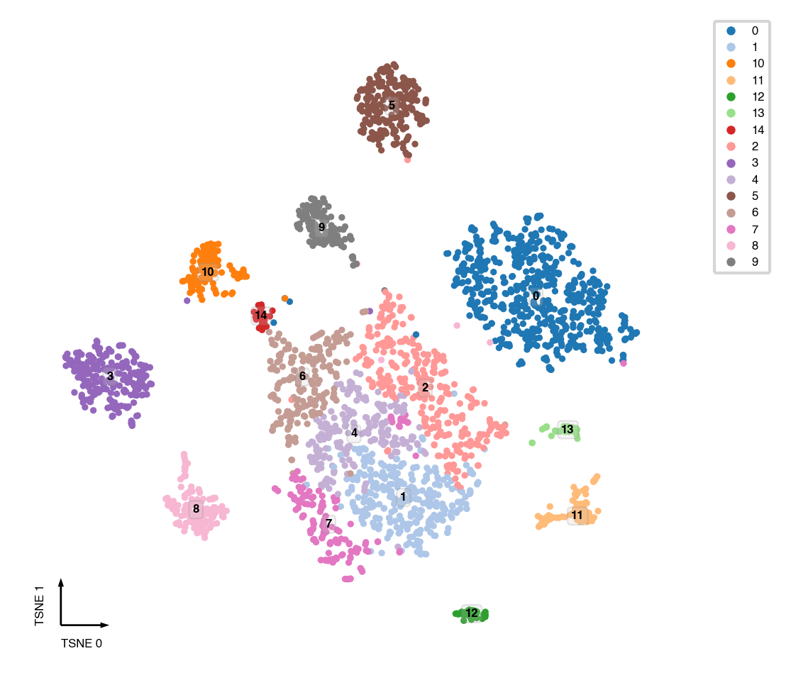
tSNE¶

tsne(mcad,
     obsm='X_pca',
     metric='euclidean',
     exaggeration=-1,  # auto determined
     perplexity=30,
     n_jobs=-1)

fig, ax = plt.subplots(figsize=(4, 4), dpi=300)
_ = categorical_scatter(data=mcad,
                        ax=ax,
                        coord_base='tsne',
                        hue='leiden',
                        text_anno='leiden',
                        show_legend=True)

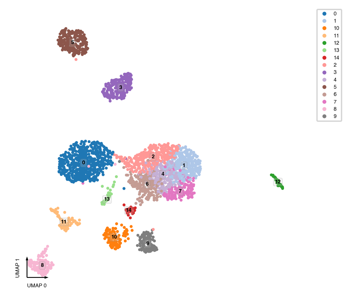
UMAP¶

sc.tl.umap(mcad)

fig, ax = plt.subplots(figsize=(4, 4), dpi=300)
_ = categorical_scatter(data=mcad,
                        ax=ax,
                        coord_base='umap',
                        hue='leiden',
                        text_anno='leiden',
                        show_legend=True)

Interactive plot¶

interactive_scatter(data=mcad, hue='leiden', coord_base='umap')

Save results¶

mcad.write_h5ad('PIT.mCG-5K-clustering.h5ad')
mcad

mcad.obs.to_csv('PIT.ClusteringResults.csv.gz')
mcad.obs.head()

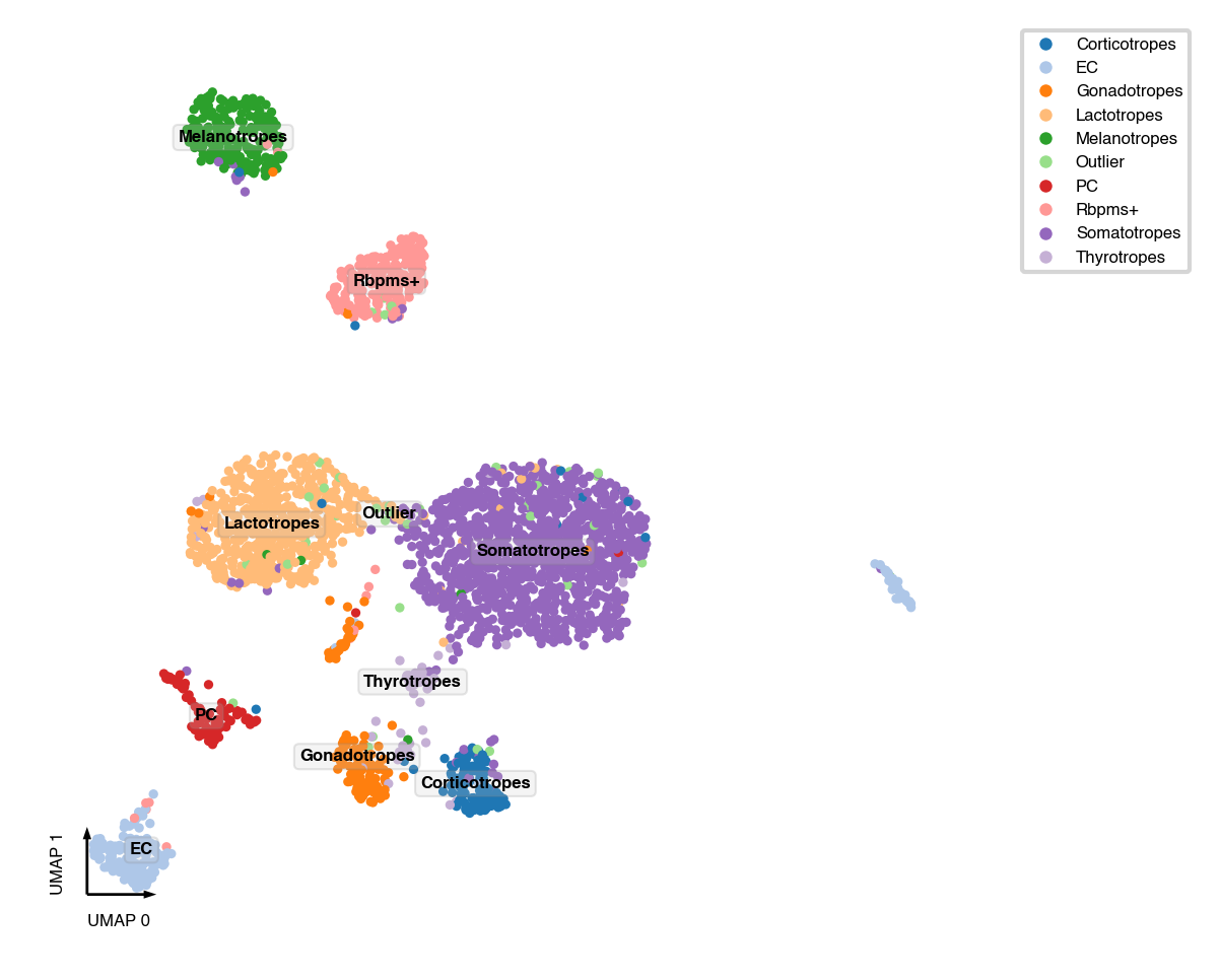
Sanity test¶

This test dataset come from [Ruf-Zamojski et al., 2021], so we already annotated the cell types. For new datasets, see following notebooks about identifying cluster markers and annotate clusters

if 'CellTypeAnno' in mcad.obs:
    mcad.obs['CellTypeAnno'] = mcad.obs['CellTypeAnno'].fillna('Outlier')
    
    fig, ax = plt.subplots(figsize=(4, 4), dpi=300)
    _ = categorical_scatter(data=mcad,
                            ax=ax,
                            coord_base='umap',
                            hue='CellTypeAnno',
                            text_anno='CellTypeAnno',
                            palette='tab20',
                            show_legend=True)

Basic Cell Clustering Using mCG-5Kb Bins

Contents